Fee estimation for light-clients (Part 3)
This post is part 3 of 3 of a series. (Part 1, Part 2)
# The model
The code building and training the model with tensorflow (opens new window) is available in google colab notebook (opens new window) (jupyter notebook); you can also download the file as plain python and run it locally. At least 1 hour is needed to train the full model, but it heavily depends on the hardware available.
As a reference, in the code we have a calculation of the bitcoin core estimatesmartfee MAE[1] and drift[2].
MAE is computed as avg(abs(fee_rate - core_econ)) when core_econ is available (about 1.2M observations, sometime the value is not available when considered too old).
| estimatesmartfee mode | MAE [satoshi/vbytes] | drift |
|---|---|---|
| economic | 28.77 | 20.79 |
| conservative | 46.49 | 44.73 |
As seen from the table, the error is quite high, but the positive drift suggests estimatesmartfee prefers to overestimate to avoid transactions not confirming.
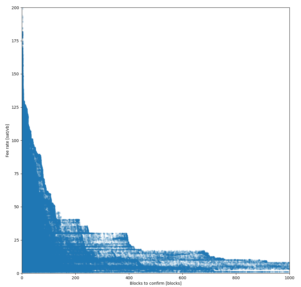
As we said in the introduction, network traffic is correlated with time and we have the timestamp of when the transaction has been first seen, however a ML model doesn't like plain numbers too much, but it behaves better with "number that repeats", like categories, so we are converting the timestamp in day_of_week a number from 0 to 6, and hours a number from 0 to 24.
# Splitting
The dataset is splitted in training and test data with a 80/20 proportion. As the name suggest the training part is used to train the model, the test is composed of other observations to test if the model is good with observations that has never seen (proving the model can generalize, not just memorizing the answer).
During the training the data is splitted again in 80/20 for training and validation respectively, validation is basically testing during training.
During splitting, the dataset is converted from a pandas data frame to tensorflow dataset, decreasing training times.
# Preprocessing
The preprocessing phase is part of the model however it contains transformations without parameters trained by the model. This transformations are useful because model trains better if data are in some format, and having this phase inside the model helps to avoid to prepare the data before feeding the model at prediction phase.
Our model performs 2 kind of preprocessing:
Normalization: model trains faster if numerical features have mean 0 and standard deviation equal to 1, so this layer is built by computing the
meanandstdfrom the series of a feature before training, and the model is feed with(feature - mean)/std. Our model normalizeconfirms_infeature and all the bucketsa*one-hot vector: Numerical categories having a small number of different unique values like our
day_of_weekandhourscould be trained better/faster by being converted in one hot vector. For exampleday_of_week=6(Sunday) is converted in a vector['0', '0', '0', '0', '0', '0', '1']whileday_of_week=5(Saturday) is converted in the vector['0', '0', '0', '0', '0', '1', '0']
# Build
all_features = tf.keras.layers.concatenate(encoded_features)
x = tf.keras.layers.Dense(64, activation="relu")(all_features)
x = tf.keras.layers.Dense(64, activation="relu")(x)
output = tf.keras.layers.Dense(1, activation=clip)(x)
model = tf.keras.Model(all_inputs, output)
optimizer = tf.optimizers.Adam(learning_rate=0.01)
model.compile(loss='mse',
              optimizer=optimizer,
              metrics=['mae', 'mse'])
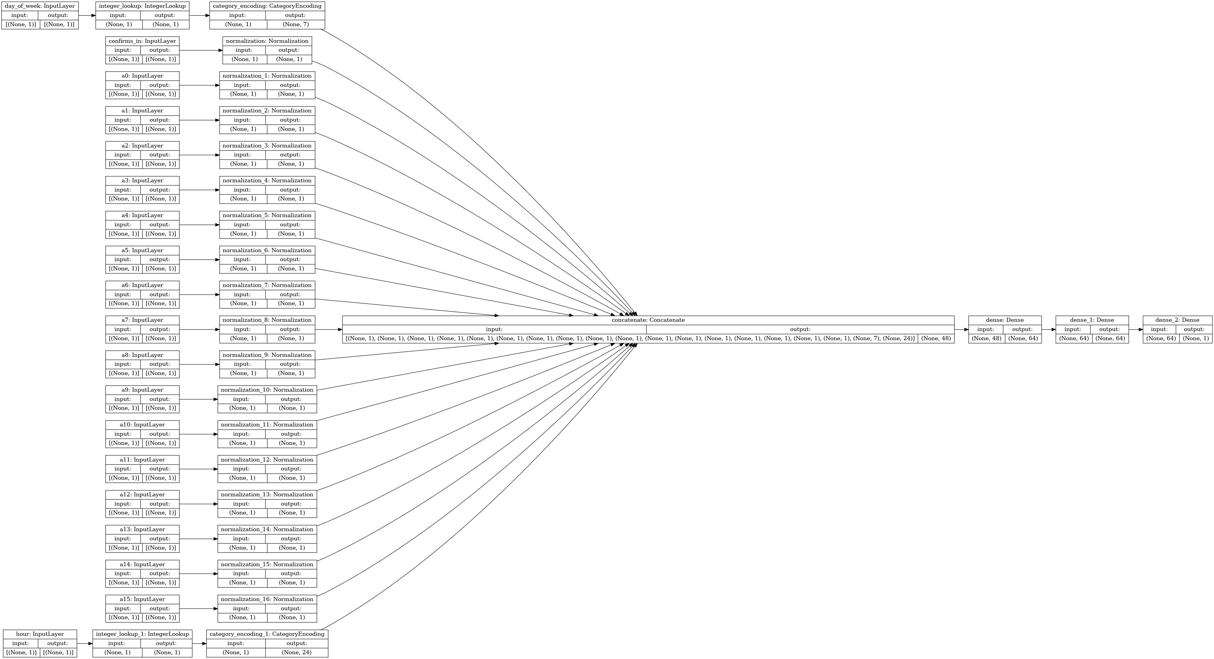
The model is fed with the encoded_features coming from the processing phase, then there are 2 layers with 64 neurons each followed by one neuron giving the fee_rate as output.
With this configurations the model has:
- Total params:
7,412 - Trainable params:
7,361 - Non-trainable params:
51
Non-trainable params comes from the normalization layer and are computed in the pre-processing phase (it contains, for example, the mean of a series). Trainable parameters are values initialized randomly and changed during the training phase. The trainable parameters are 7,361, this number comes from the following, every neuron has an associated bias and a weight for every element in the inputs, thus:
(48 input_values_weights + 1 bias) * (64 first_layer_neurons)
+ (64 input_values_weights + 1 bias) * (64 second layer neurons)
+ (64 input values weights + 1 bias)

49*64+65*64+65 = 7361
Honestly, neural network parameters are mostly the one taken from this tensorflow example (opens new window), we even tried to tune hyperparameters (opens new window), however, we decided to follow this advice (opens new window): "The simplest way to prevent overfitting is to start with a small model:". We hope this work will attract other data scientists to this bitcoin problem, improving the model. We also think that a longer time for the data collection is needed to capture various situations.
A significant part of a ML model are the activation functions, relu (Rectified Linear Unit) is one of the most used lately, because it's simple and works well as we learned in this introducing neural network video (opens new window). relu it's equal to zero for negative values and equal to the input for positive values. Being non-linear allows the whole model to be non-linear.
For the last layer it is different: we want to enforce a minimum for the output, which is the minimum relay fee 1.0[3]. One could not simply cut the output of the model after prediction because all the training would not consider this constraint. So we need to build a custom activation function that the model training will be able to use for the gradient descent (opens new window) optimization step. Luckily this is very simple using tensorflow primitives:
def clip(x):
  min = tf.constant(1.0)
  return tf.where(tf.less(x, min), min, x)
Another important part is the optimizer, when we first read the aforementioned example (opens new window) the optimizer used was RMSProp however the example updated lately and we noticed the optimizer changed in favor of Adam which we read is the latest trend (opens new window) in data science. We changed the model to use Adam and effectively the training is faster with Adam and even slightly lower error is achieved.
Another important parameter is the learning rate, which we set to 0.01 after manual trials; however there might be space for improvements such as using exponential decay (opens new window), starting with an high learning rate and decreasing it through training epochs.
The last part of the model configuration is the loss function: the objective of the training is to find the minimum of this function. Usually for regression problem (the ones having a number as output, not a category) the most used is the Mean squared error (MSE). MSE is measured as the average of squared difference between predictions and actual observations, giving larger penalties to large difference because of the square. An interesting property is that the bigger the error the faster the changes is good at the beginning of the training, while slowing down when the model predicts better is desirable to avoid "jumping out" the local minimum.
# Finally, the model training
PATIENCE = 20
MAX_EPOCHS = 200

def train():
  early_stop = keras.callbacks.EarlyStopping(monitor='val_loss', patience=PATIENCE)
  history = model.fit(train_ds, epochs=MAX_EPOCHS, validation_data=val_ds, verbose=1, callbacks=[early_stop])
  return history

history = train()
This steps is the core of the neural network, it takes a while, let's analyze the output:
Epoch 1/200
7559/7559 [==============================] - 34s 3ms/step - loss: 547.8023 - mae: 16.9547 - mse: 547.8023 - val_loss: 300.5965 - val_ma
e: 11.9202 - val_mse: 300.5965
...
Epoch 158/200
7559/7559 [==============================] - 31s 3ms/step - loss: 163.2548 - mae: 8.3126 - mse: 163.2548 - val_loss: 164.8296 - val_mae: 8.3402 - val_mse: 164.8296
Training is done in epochs, under every epoch all the training data is iterated and model parameters updated to minimize the loss function.
The number 7559 represent the number of steps. Theoretically the whole training data should be processed at once and parameters updated accordingly, however in practice this is infeasible for example for memory resource, thus the training happens in batch. In our case we have 1,934,999 observations in the training set and our batch size is 256, thus we have 1,437,841/256=7,558.58 which by excess result in 7559 steps.
The ~31s is the time it takes to process the epoch on a threadripper CPU but GPU or TPU could do better.
The value loss is the MSE on the training data while val_loss is the MSE value on the validation data. As far as we understand the separated validation data helps to detect the machine learning enemy, overfitting. Because in case of overfitting the value loss continue to improve (almost indefinitely) while val_loss start improving with the loss but a certain point diverge, indicating the network is memorizing the training data to improve loss but in doing so losing generalizing capabilities.
Our model doesn't look to suffer overfitting cause loss and val_loss doesn't diverge during training
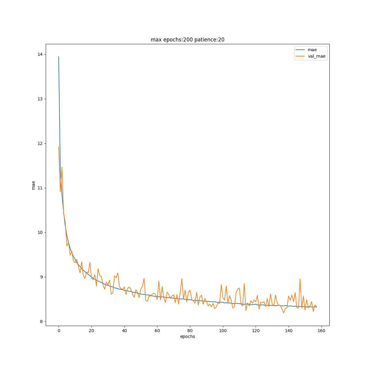
While we told the training to do 200 epochs, the training stopped at 158 because we added an early_stop call back with 20 as PATIENCE, meaning that after 20 epoch and no improvement in val_loss the training is halted, saving time and potentially avoiding overfitting.
# The prediction phase
A prediction test tool (opens new window) is available on github. At the moment it uses a bitcoin core node to provide network data for simplicity, but it queries it only for the mempool and the last 6 blocks, so it's something that also a light-client could do[4].
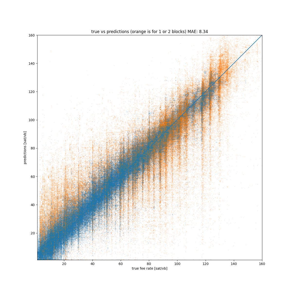
The following chart is probably the best visualization to evaluate the model, on the x axis there is the real fee rate while on the y axis there is the prediction, the more the points are centered on the bisection, the more the model is good.
We can see the model is doing quite well, the MAE is 8 which is way lower than estimatesmartfee. However, there are big errors some times, in particular for prediction for fast confirmation (confirms_in=1 or confirms_in=2) as shown by the orange points. Creating a model only for blocks target greater than 2 instead of simply remove some observations may be an option.
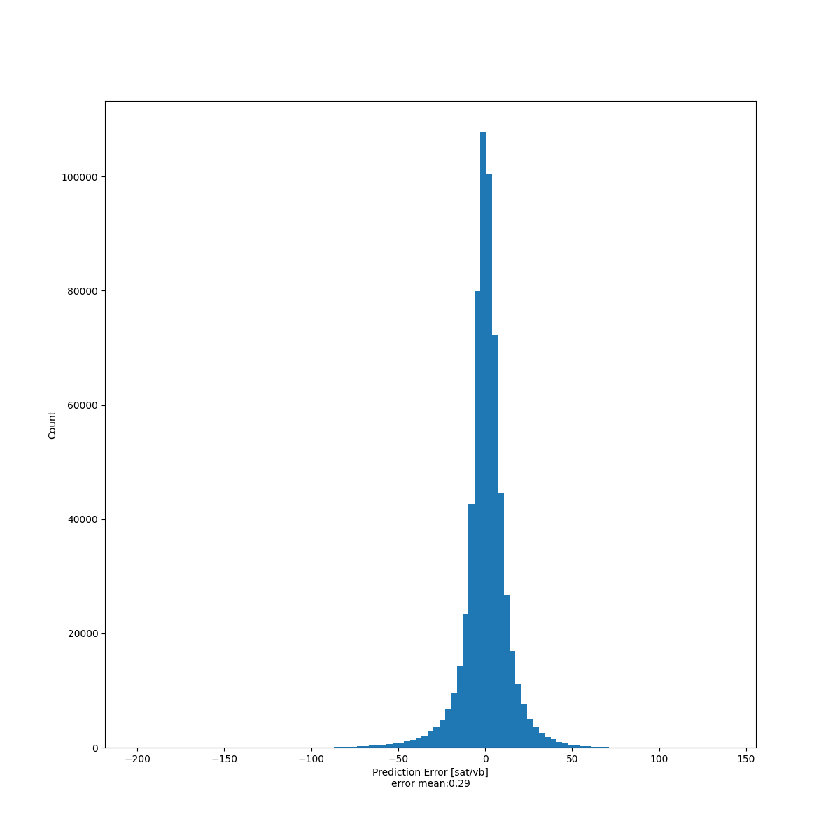
The following chart is instead a distribution of the errors, which for good model should resemble the normal distribution centered in 0, and it loooks like the model is respecting that.
# Conclusion and future development
The results have shown deep neural network are a tool capable of good bitcoin transaction fee estimations; this suggests that further ML research in this area might be promising.
This is just a starting point, there are many future improvements such as:
- Build a separate model with full knowledge, thus for full, always-connected nodes could be interesting and improve network resource allocation with respect to current estimators.
- Tensorflow is a huge dependency, and since it contains all the feature to build and train a model, most of the feature are not needed in the prediction phase. In fact tensorflow lite exists which is specifically created for embedded and mobile devices; the prediction test tool (opens new window) and the final integration in bdk (opens new window) should use it.
- Explore other fields to improve model predictions such as:
- A bucket array of the transactions in the last 6 blocks with known fee rates. This should in particular help estimations with almost empty mempool.
- Transaction weight
- Time from last block
- Some fields are very important and could benefit from pre-processing expansion, for instance applying hashed feature columns (opens new window) to
confirms_in. - Bitcoin logger could be improved by a merge command to unify raw logs files, reducing redundancy and consequently disk occupation.
- The dataset could be created in multiple files to allow more parallelism and use less memory during training.
- Saving the dataset in TFRecord format (opens new window) instead of CSV
- At the moment we are training the model on a threadripper CPU, training the code on GPU or even TPU will be needed to decrease training time, especially because input data will grow.
- The prediction test tool (opens new window) should estimate only using the p2p bitcoin network, without requiring a node. This work would be propedeutic for bdk (opens new window) integration
- At the moment mempool buckets are multiple inputs
a*as show in the model graph; since they are related, is it possible to merge them in one TensorArray? - Sometimes the model does not learn and gets stuck (opens new window). The reason is the
clipfunction applied in the last layer is constant for a value lower than 1. In this case, the derivative is 0 and the gradient descent doesn't know where to go. Instead of using theclipfunction apply penalties to the loss function for values lower than 1. - There are issues regarding dead neurons (going to 0) or neurons with big weight, weight results should be monitored for this events, and also weight decay and L2 regularization should be explored.
- Tune hyper-parameters technique should be re-tested.
- Predictions should be monotonic decreasing for growing
confirms_inparameter; for obvious reason it doesn't make sense that an higher fee rate will result in a higher confirmation time. But since this is not enforced anywhere in the model, at the moment this could happen. - Since nodes with bloom filter disabled doesn't serve the mempool anymore, a model based only on last blocks should be evaluated.
# Acknowledgements
Thanks to Square crypto (opens new window) for sponsoring this work and thanks to the reviewers: Leonardo Comandini (opens new window), Domenico Gabriele (opens new window), Alekos Filini (opens new window), Ferdinando Ametrano (opens new window).
And also this tweet that remembered me I (opens new window) had this work in my TODO list
I don't understand Machine Learning(ML), but is it horrible to use ML to predict bitcoin fees?
— sanket1729 (@sanket1729) December 9, 2020
I have heard tales of this "Deep Learning" thing where you throw a bunch of data at it and it gives you good results with high accuracy.
This is the final part of the series. In the previous Part 1 we talked about the problem and in Part 2 we talked about the dataset.
MAE is Mean Absolute Error, which is the average of the series built by the absolute difference between the real value and the estimation. ↩︎
drift like MAE, but without the absolute value ↩︎
Most node won't relay transactions with fee lower than the min relay fee, which has a default of
1.0↩︎An important issue emerged after the article came out, a bitcoin core client with bloom filter disabled (default as of 0.21) doesn't serve the mempool via p2p. ↩︎